My master's thesis: reconstructing extensive air showers detected at the HAWC observatory
My master's thesis in Artificial Intelligence (UNIR, 2024): a model based on a convolutional neural network that predicts the core position of the extensive air showers produced by cosmic rays at the HAWC observatory.
Download the full thesis80 pages · 5.8 MB · in SpanishAbstract
Cosmic rays, high-energy particles from space, hit the Earth's atmosphere and create extensive air showers, which spread out laterally and vertically and are detected by specialised observatories. HAWC, on the slope of the Sierra Negra volcano (Mexico), detects them with water Cherenkov detectors. Most of the observatory's algorithms are optimised for gamma rays, so they are not optimal for studying cosmic rays. This work proposes using artificial intelligence to build a model tailored specifically to cosmic rays, providing one of the variables needed to reconstruct the showers: the prediction of their core position.
Main results
01
Context
Cosmic rays and air showers
A primary cosmic ray is a subatomic particle that arrives from space at close to the speed of light. When it collides with a nucleus in the atmosphere it sets off a cascade of reactions: a shower of secondary particles that widens vertically and laterally until it reaches the ground. The point where the axis of that shower meets the ground is the shower's core.
How the HAWC observatory sees them
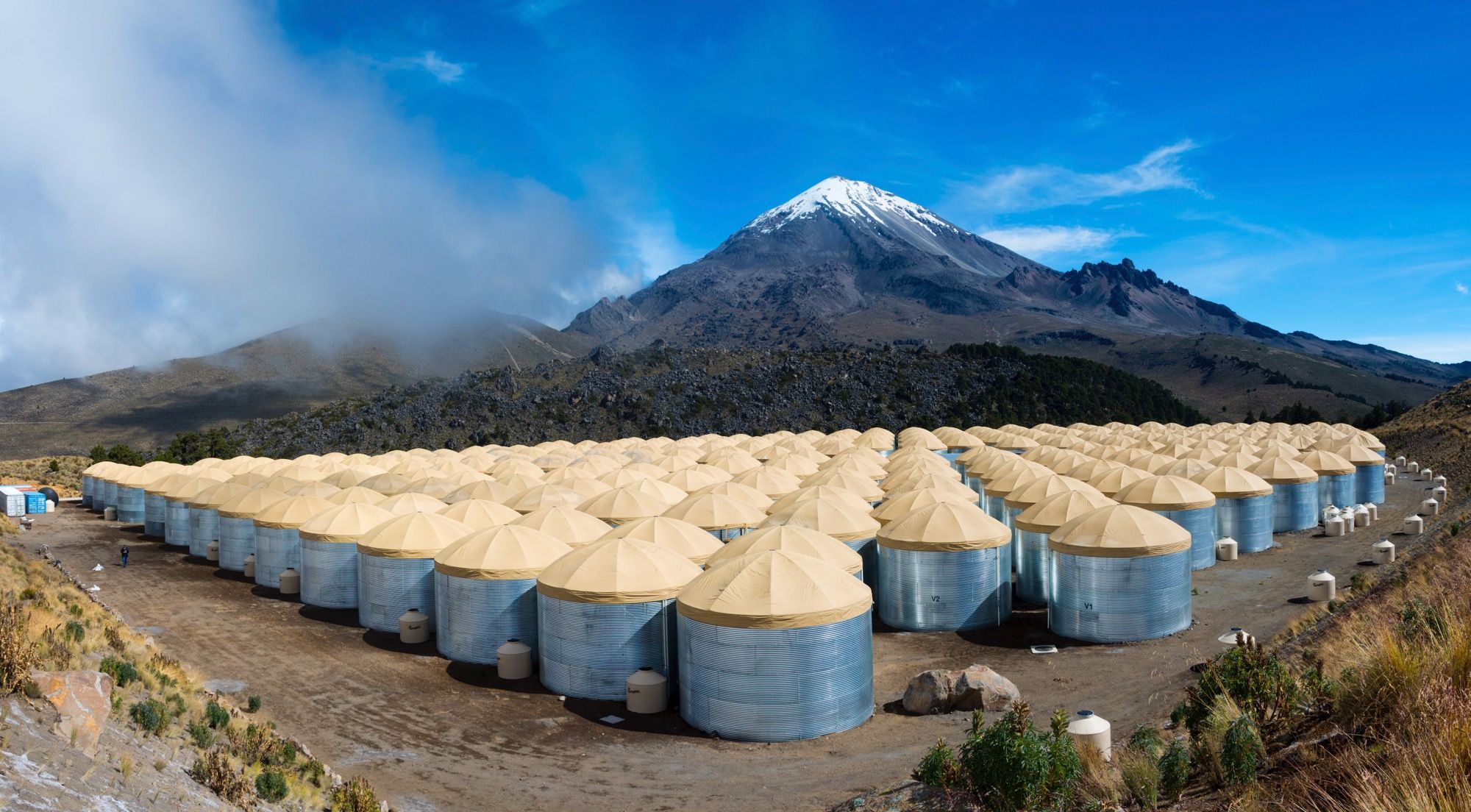
HAWC (High Altitude Water Cherenkov) sits on the slope of the Sierra Negra volcano, in Puebla (Mexico). It does not see the particles directly: it sees the light they emit as they cross the water in its tanks. When a charged particle travels through a medium faster than light does in that medium, it emits a cone of light: this is the Cherenkov effect.
| Altitude | 4,100 m |
|---|---|
| Detectors | 300 tanks in a grid |
| Area | ~22,000 m² |
| Tank | 7.3 m × 4.5 m, steel |
| Water | 180,000 l, ultrapure |
| Sensors | 4 PMTs per tank, at ~4 m |
The problem
Locating the core is the first step of the reconstruction: the energy and direction of the primary depend on it, and with them the measurement of the cosmic-ray spectrum. But HAWC is optimised for gamma rays, its main line of research. Cosmic-ray showers are different: sensors far from the core can record sub-showers, which does not happen with gammas.
The result is a systematic error. With the current algorithm, the core of cosmic-ray showers comes out shifted by 94.6 m in X and 262.3 m in Y on average. On top of that, many showers fall partly outside the area covered by the tanks, and their core still has to be estimated.
02
Method
Data
Training requires knowing where the core really landed, and real data does not tell you that. So the model learns from events simulated by the observatory's own software, stored in XCDF files. The positions of the tanks and their sensors come from HAWC's survey.xml file.
Before going into training, each event passes a filter: valid reconstruction, angle and core (status = 0), more than 75 hits and a ratio of hits to available channels above 0.22. The final set has 4 million events, with angles between 0 and 0.60 rad and between 0 and 1,200 hits.
From an event to an image
The tanks are laid out in a grid and each one holds 4 PMT sensors, so the information of each event can be represented much like an image. Each tank takes up a 2 × 2 submatrix within a 40 × 30 matrix, and the different values of each PMT are stored in separate layers, just as RGB images store each colour in a layer.
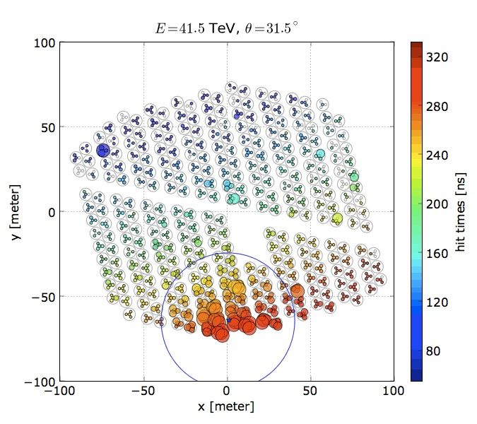
The four layers are the energy, the zenith angle of the shower (the same for the whole event) and the X and Y position of each sensor relative to the centre of the observatory. Only cells with a hit carry values. Building the set costs O(n × m), with n events and m hits per event: the position of each hit in the matrix is computed in O(1).
Architecture
The goal is to predict spatial values, the coordinates of a position on a plane, and the input represents values on that same plane. That is why a convolutional neural network was chosen: it combines Conv2D layers with MaxPooling, followed by a dense layer that predicts the coordinates by linear regression.
| Layer | Configuration | Purpose |
|---|---|---|
| Conv2D | 128 filters 3 × 3 · Leaky ReLU | Detects spatial patterns |
| MaxPooling2D | 2 × 2 | Reduces dimensionality while keeping what matters most |
| Conv2D | 256 filters 3 × 3 · Leaky ReLU | Detects spatial patterns |
| MaxPooling2D | 2 × 2 | — |
| Conv2D | 256 filters 3 × 3 · Leaky ReLU | — |
| Flatten + Dense | 256 neurons · Leaky ReLU | Turns the maps into a vector and processes it |
| Dense | 2 · linear | Predicts the (x, y) coordinates by linear regression |
Unlike ReLU, Leaky ReLU does not turn negative values into zero: it scales them by a small factor. That avoids vanishing gradients, which matters when the input data contains relevant negative values.
Training
The model was trained for 30 epochs, tracking the loss and the mean absolute error (MAE). On the training set both go down steadily. On validation they stall early and oscillate.
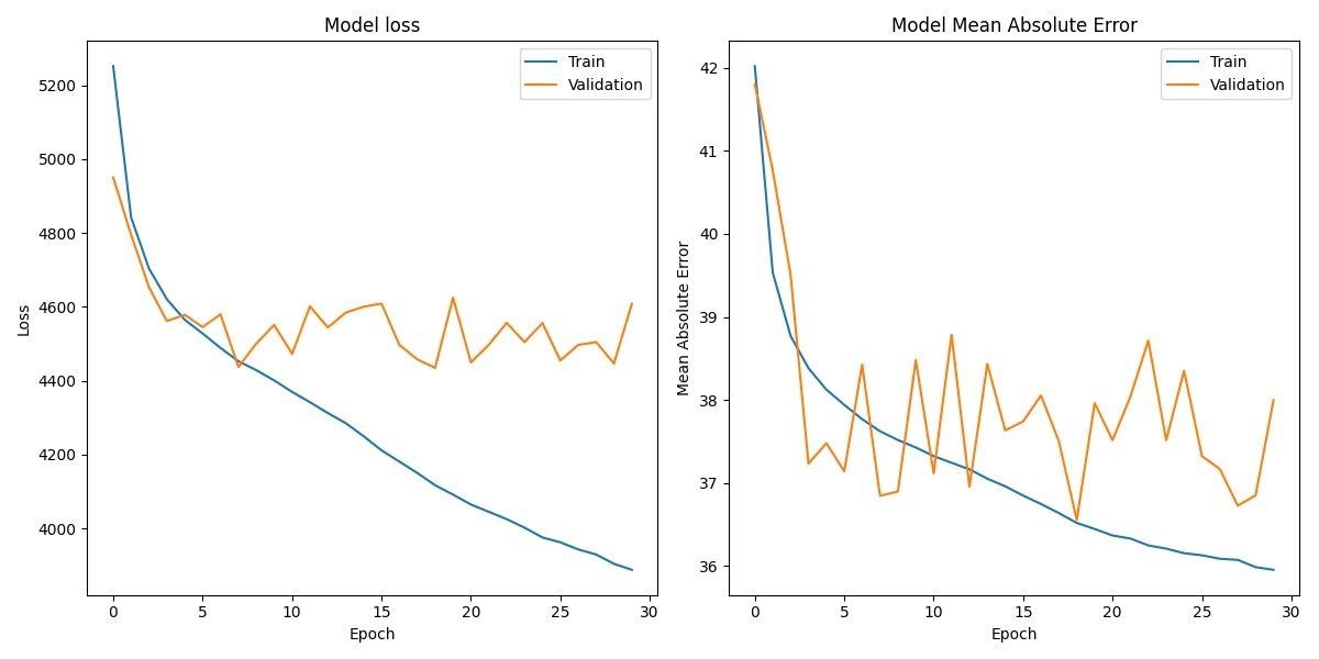
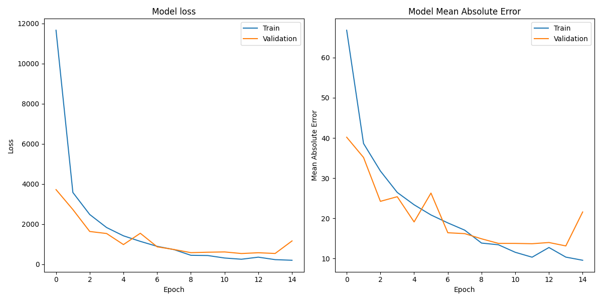
To test that hypothesis I repeated the training with 1,000 similar events: angles between 0.45 and 0.50 rad and between 600 and 800 hits. With homogeneous data, the validation metrics behave much more like the training ones, and the training ones are significantly better. The thesis puts the stalling down to the high variability of the data: one event can be very different from another because of its position in the observatory, the energy of each hit or its inclination.
03
Results
Does it get the distance to the centre right?
To compare the prediction with the true value at a glance, the distance from the core to the centre of the observatory is used, r = √(x² + y²). If the model were perfect, every event would fall on the diagonal y = x.
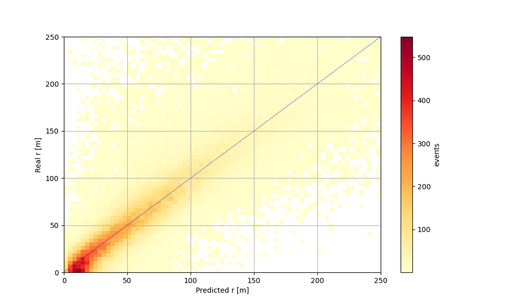
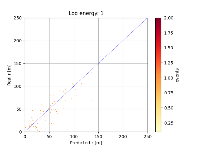
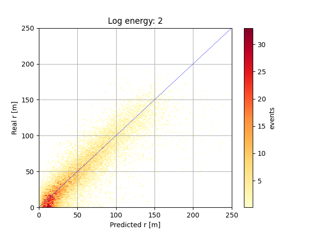
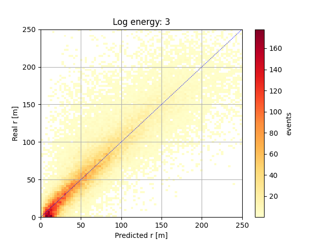
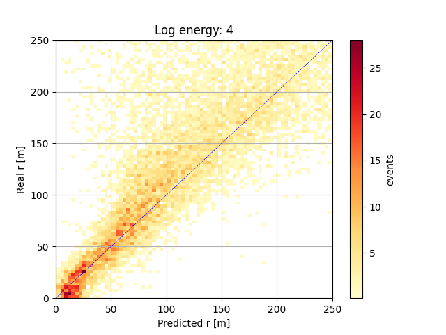
Most events sit on the diagonal, especially near the centre. The spread grows with distance and with energy: the further away the core lands, the less information reaches the tanks.
Precision: the spread of the error
For each event the true coordinate is subtracted from the predicted one and a Gaussian is fitted to those differences. Its width, σ, measures the precision: the lower, the better.
| log E | σ X HAWC | σ X network | Improvement | σ Y HAWC | σ Y network | Improvement |
|---|---|---|---|---|---|---|
| All | 61.1 | 37.7 | −38% | 62.5 | 38.5 | −38% |
| 1–2 | 69.3 | 17.6 | −75% | 68.0 | 17.9 | −74% |
| 2–3 | 48.5 | 19.8 | −59% | 50.9 | 18.7 | −63% |
| 3–4 | 52.6 | 28.5 | −46% | 53.7 | 29.0 | −46% |
| 4–5 | 101.3 | 72.5 | −28% | 102.4 | 75.5 | −26% |
σ in metres. Table 6 of the thesis; the improvement is (1 − σ network / σ HAWC).
Bias: where the error is centred
The mean of those differences tells you whether the model always errs in the same direction. This is where the two methods differ most clearly.
HAWC's algorithm shifts the core by about 93 m in X and about 262 m in Y at every energy level. The network stays centred on zero: between −3.4 and 0.3 m in every case except X at the highest energies (−12.4 m).
04
Conclusions
- Goal. Improve the prediction of the core coordinates of the extensive air showers detected at the HAWC observatory.
- Methodology. A convolutional neural network that, without having images of the events, arranges their data in matrices that mirror the geographical layout of the sensors, with each detector's parameters in layers, as in colour images.
- Results. The model predicts the coordinates more precisely than HAWC's current model, with a significant reduction in error, especially for events with a log energy below 4. HAWC's model shows larger errors at every energy level.
- Conclusion. The convolutional neural network outperforms HAWC's model in precision, validated with histograms and visual comparisons.
Future work
Two lines: training with more resources and more events, and training several models specialised in similar events (by arrival angle, energy and number of hits), choosing the most suitable one for each case at prediction time.
Read the full thesis
The 80 pages cover the background on high-energy astronomy and machine learning, the requirements and design of the tool, the full evaluation and the per-energy histograms in the appendices.
Download the PDF (5.8 MB, in Spanish) ↓Technical details and how to cite it
Stack: Python 3, TensorFlow/Keras, scikit-learn, XCDF, Matplotlib.
How to cite: Galán Triguero, D. (2024). Reconstrucción de cascadas atmosféricas extendidas detectadas en observatorio HAWC [Master's thesis, Máster Universitario en Inteligencia Artificial]. Universidad Internacional de La Rioja.
If you'd like to talk about it, write to me.